Understanding Sound Pressure Level

Sound pressure level (SPL) is a ratio measure of the pressure of a sound wave in relation to a reference pressure. SPL has a logarithmic scale, and is measured in decibels (which is also a logarithmic ratio measurement, the details of which can be found here.) We can think about SPL as a measure of loudness, often used to monitor environmental sound levels, or in product testing to measure the output of a specific device like a loudspeaker or headphones. It is a very useful measurement to moderate the safety of a given room or system. Generally the lowest SPL we can perceive is about 0 dB_SPL, with exposure to levels above 85 dB_SPL considered potentially harmful and above 140 dB_SPL unsafe. The following figure displays sound pressure levels of common sonic events.

The problem with the diagram above is that it does not specify at what distance from these sonic events SPL is measured. SPL, in this case, is calculated from an estimated 'normal' distance for each situation. For example, you may be one meter away from your conversation partner, but 100 meters away from an airplane lift-off. We all know that when you move away from a sound source, you perceive the source as less loud; in audio we often describe this effect using the ‘Inverse Distance’ of ‘1/r’ Law. The law governs, as the distance from a sound source is doubled, its SPL is attenuated 6 decibels. This may seem intuitive, but actually as the measuring distance is increasing exponentially, SPL is decreasing linearly. This is explained by  SPL’s logarithmic nature. It is also important to note that this law is only accurate in a free field. In a room with reflections, SPL would decrease even less because the reflections increase SPL level.

Now that we have established a basic idea of SPL and what it is used for, we can begin to untangle its calculation. The formula is as follows:

To use this formula we need ‘p’ and ‘p_ref’. Lower case ‘p’ is the pressure in Pascal that we measure from a sound source, and p_ref is a (somewhat) constant reference pressure. Generally, SPL is calculated with a reference pressure of 20 uPa, which is approximately the lower threshold of human hearing. So, the calculation for SPL at a single point in time is quite straightforward. However, sound happens over time, and it is useful to be able to measure the SPL continuously.

To calculate SPL over time one could use a Sound Pressure Level Meter, usually a handheld device that is calibrated to display accurate SPL continuously using internal calculations. However, it is also possible to create an SPL meter in any programming language using some filters, a few calculations, and a loop or two. The following section focuses on how to implement and interpret the many different methods of SPL calculation, generally displayed as a graph of SPL over time.

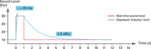
To get from a single SPL measurement to a curve displaying continuous SPL, the first step is to choose a time-weighting. Time-weighting controls how many times per second SPL is sampled, with the purpose of capturing the most important aspects of a given signal. Technically, one could choose any time period with which to sample, but the most common are "fast", "slow", and "impulse" weighting. Fast-weighting samples SPL every 125 ms, and is most representative of the measured sound as it happened in air. However, for a rapidly changing signal, slow-weighting, which samples once per second, is often desirable to create a more smooth, readable curve. Impulse-weighting reacts very quickly to the onset of a sound (35 ms), but decays slowly, making it useful for impulse type measurements. All of these weightings also employ a certain overlap period to avoid sharp jumps in the resulting figure. The following figures (source: NTi Audio) show how different time weightings would display a sonic event.

Next, one must choose a frequency weighting. Frequency-weightings are used to display SPL as it is perceived by the human ear. Due to the shape of the ear canal, and exposure to important sonic events, humans are most sensitive to frequencies between 2 - 4 kHz, perceiving them as louder. Even within the range of human hearing (20 Hz - 20 kHz), we perceive very high and very low frequencies as significantly less loud, especially when they occur with a lower amplitude. "A-weighting" takes into account these idiosyncrasies of human hearing and damps the SPL of low and high frequencies with a slight boost in the mid-range. "C-weighting" has a similar effect but attenuates the lower frequencies less to be more representative of very loud events, since the human ear is quite reactive in this case. "Z-weighting" ("zero") makes no frequency-dependent changes to SPL . The following figure from NTi Audio shows how each weighting type would affect the amplitude of SPL at a given frequency.

Once one of these weightings is applied to a series of discrete SPL calculations, a continuous curve can be calculated using the averaging method Root Mean Square (RMS). RMS takes the square root of the mean of the square of a pressure signal over a duration of time (see formula below). It is found to be an accurate way to display the energy of a pressure wave in time. We should note once again, RMS is not just calculated between time-weighting defined points, but with a small window of overlap for accuracy and legibility of the curve.

p_{RMS}=\sqrt{\frac{1}{T}\int_{t_{0}}^{t_{0+T}}p(t)^2 dt}

The last variation to be discussed is

L_{eq}

, sometimes referred to as

L_{AT}

, which stands for Equivalent Continuous SPL and time-averaged SPL respectively.

L_{eq}

is a single number that represents the SPL that produces the same amount of energy as the original signal over a given time frame. Therefore, it is a measure of average energy from the original signal. It is calculated as the RMS value with measurement duration as "averaging" (integration) time.

L_{eq}

can be calculated with any frequency-weighting. The following figure, provided by NTi Audio, shows Equivalent Continuous SPL as the red line calculated over a measurement period of 5 minutes.

The final table provides a key for the common notation of the different calculation methods described above; it is not exhaustive, but meant to provide examples of how the different weightings can be combined. Note that 'L' stands for level in each of tese terms.